Note: This notebook was created largely based off Preprocessing and clustering 3k PBMCs. Portions have been removed/edited to adapt to a class time of ~30 minutes.
scanpy is a toolkit based in python for single-cell analysis. Some applications of scanpy include:
clustering of single-cell data
trajectory inference (reconstruction of cell pathways)
differential expression testing (testing differences in gene expression between different cell populations)
Learning objectives
Gain familiarity with single-cell data
Experiment with the adata object
Perform dimension reduction and some clustering analysis of scRNA-seq
Let’s first discuss what single-cell data is/looks like…
single-cell data
There are several types of single-cell data:
scDNA-seq (genomic single-cell)
scRNA-seq (transcriptomic single-cell)
scBS-seq (single-cell bisulfite sequencing)
…
These modalities differentiate biological behavior/mechanisms. In this tutorial, we will be looking at 2700 peripheral blood mononuclear cells (PBMCs) from a healthy donor.
What are the benefits of single-cell sequencing over bulk sequencing?
Knowing the sequencing profiles of single-cells adds granularity to data obtained from samples that may contain more than one type of cell. For instance, knowing the transcriptomic profiles of single cells in a population of heterogeneous tumor cells can reveal insights into tumorigenesis. Researchers may be able to investigate novel biological activity as stem cells abnormally mature into cancerous cells.
How is single-cell data created?
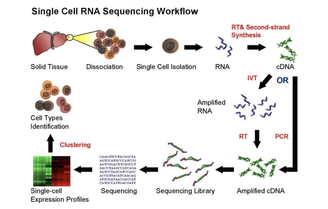
There are various methods depending on the application and type of single-cell data. However, I hope the image (Chan Zuckerberg Initiative) below captures how single-cell data is created. In short, single cells are isolated from tissue, sequenced and amplified.
scRNA-seq workflow
Now that we know how single-cell data is generated, let’s talk about how single-cell data is represented in scanpy.
# install these packages first# install the anndata library!pip install anndata# install the scanpy library!pip install scanpy!pip install leidenalg
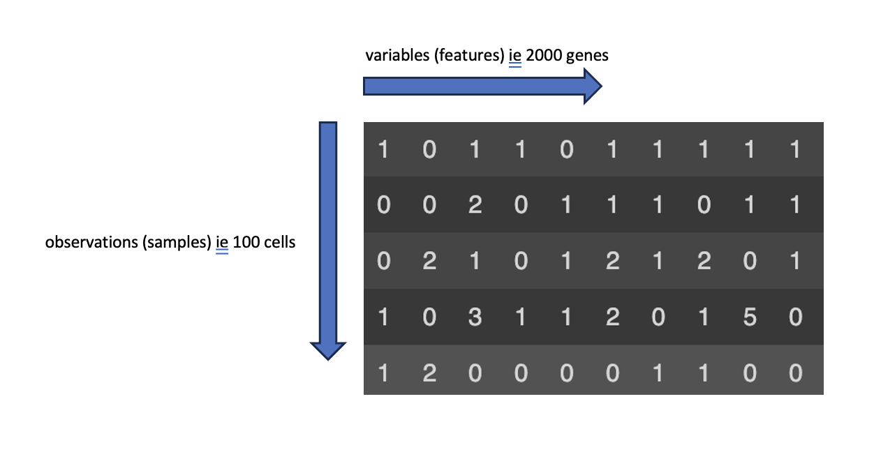
The anndata python package enables the use of anndata objects which are essentially annotated data matrices.
The following (taken from Getting started with anndata) demonstrates some of the features of the anndata object.
# first, create a matrix of 100 (cells) x 2000 (genes)counts = csr_matrix(np.random.poisson(1, size=(100, 2000)), dtype=np.float32)adata = ad.AnnData(counts)# create index names...observation names and variable namesadata.obs_names = [f"Cell_{i:d}"for i inrange(adata.n_obs)]adata.var_names = [f"Gene_{i:d}"for i inrange(adata.n_vars)]print(adata.obs_names[:10])
After running the code above, the adata object created has a data matrix X attribute which essentially looks like the below:
adata object
This can also be observed in python by running the below which converts the aData object into a dataframe using to_df.
# outputs a dataframe version of the X matrixadata.to_df()
Gene_0
Gene_1
Gene_2
Gene_3
Gene_4
Gene_5
Gene_6
Gene_7
Gene_8
Gene_9
...
Gene_1990
Gene_1991
Gene_1992
Gene_1993
Gene_1994
Gene_1995
Gene_1996
Gene_1997
Gene_1998
Gene_1999
Cell_0
0.0
2.0
0.0
2.0
2.0
0.0
0.0
1.0
1.0
1.0
...
1.0
2.0
2.0
0.0
1.0
2.0
3.0
1.0
1.0
1.0
Cell_1
0.0
1.0
1.0
1.0
0.0
1.0
3.0
0.0
1.0
0.0
...
0.0
1.0
2.0
2.0
1.0
1.0
1.0
1.0
2.0
0.0
Cell_2
0.0
1.0
0.0
2.0
1.0
2.0
2.0
0.0
3.0
1.0
...
1.0
2.0
1.0
0.0
1.0
2.0
2.0
1.0
0.0
2.0
Cell_3
0.0
2.0
2.0
0.0
2.0
1.0
2.0
0.0
1.0
2.0
...
0.0
2.0
2.0
2.0
2.0
2.0
1.0
2.0
0.0
2.0
Cell_4
0.0
0.0
0.0
1.0
1.0
1.0
1.0
2.0
2.0
0.0
...
0.0
2.0
2.0
1.0
1.0
0.0
1.0
0.0
1.0
0.0
...
...
...
...
...
...
...
...
...
...
...
...
...
...
...
...
...
...
...
...
...
...
Cell_95
0.0
1.0
0.0
2.0
1.0
0.0
2.0
1.0
0.0
0.0
...
1.0
0.0
2.0
1.0
1.0
1.0
0.0
0.0
0.0
0.0
Cell_96
3.0
1.0
0.0
3.0
1.0
1.0
0.0
0.0
2.0
0.0
...
0.0
2.0
1.0
1.0
1.0
2.0
0.0
0.0
1.0
0.0
Cell_97
0.0
0.0
1.0
0.0
5.0
0.0
1.0
2.0
2.0
1.0
...
1.0
0.0
1.0
1.0
1.0
2.0
0.0
1.0
1.0
2.0
Cell_98
0.0
1.0
2.0
1.0
2.0
2.0
1.0
0.0
1.0
1.0
...
1.0
2.0
0.0
2.0
0.0
1.0
0.0
0.0
2.0
1.0
Cell_99
1.0
2.0
1.0
2.0
1.0
0.0
1.0
0.0
2.0
1.0
...
1.0
2.0
2.0
0.0
3.0
0.0
1.0
2.0
0.0
3.0
100 rows × 2000 columns
Now, let’s add in some annotations/metadata at the observation level. This could be the cell type of each observation.
# random cell assignmentct = np.random.choice(["B", "T", "Monocyte"], size=(adata.n_obs,))adata.obs["cell_type"] = pd.Categorical(ct) # Categoricals are preferred for efficiencyadata.obs
cell_type
Cell_0
Monocyte
Cell_1
T
Cell_2
B
Cell_3
T
Cell_4
B
...
...
Cell_95
B
Cell_96
Monocyte
Cell_97
B
Cell_98
B
Cell_99
B
100 rows × 1 columns
For metadata that has many dimensions (each cell could have a 2-dim UMAP mapping or each gene could have a 5-dim feature set), we can use the obsm and varm attributes as shown below.
The above is a very brief overview of the anndata object. For more information, see Getting started with anndata.
Let’s move on to some of the functions of scanpy.
# scanpy demo
First, let’s download and read in the demo 3k PBMC scRNA-seq data from 10X Genomics (company that provides services single-cell data generation and analysis).
# fetch the scanpy demo data!mkdir data!wget http://cf.10xgenomics.com/samples/cell-exp/1.1.0/pbmc3k/pbmc3k_filtered_gene_bc_matrices.tar.gz -O data/pbmc3k_filtered_gene_bc_matrices.tar.gz!cd data; tar -xzf pbmc3k_filtered_gene_bc_matrices.tar.gz# read in the data# place cursor after first parantheses and push ctrl/cmd+shift+space bar to bring up docstringsadata = sc.read_10x_mtx('data/filtered_gene_bc_matrices/hg19/', # the directory with the `.mtx` file var_names='gene_symbols', # use gene symbols for the variable names (variables-axis index) cache=True) # write a cache file for faster subsequent reading
---------------------------------------------------------------------------NameError Traceback (most recent call last)
CellIn[7], line 8 4 get_ipython().system('cd data; tar -xzf pbmc3k_filtered_gene_bc_matrices.tar.gz')
6# read in the data 7# place cursor after first parantheses and push ctrl/cmd+shift+space bar to bring up docstrings----> 8 adata = sc.read_10x_mtx(
9'data/filtered_gene_bc_matrices/hg19/', # the directory with the `.mtx` file 10 var_names='gene_symbols', # use gene symbols for the variable names (variables-axis index) 11 cache=True) # write a cache file for faster subsequent readingNameError: name 'sc' is not defined
scanpy - explore and filter data
Let’s first look at the most highly expressed 20 genes in our dataset:
sc.pl.highest_expr_genes(adata, n_top=20, )# return the number of observationsprint(adata.n_obs)# return the number of variablesprint(adata.n_vars)
---------------------------------------------------------------------------NameError Traceback (most recent call last)
CellIn[8], line 1----> 1sc.pl.highest_expr_genes(adata, n_top=20, )
2# return the number of observations 3print(adata.n_obs)
NameError: name 'sc' is not defined
Now, let’s do some filtering for gene and cell representation.
sc.pp.filter_cells(adata, min_genes=200)sc.pp.filter_genes(adata, min_cells=3)# return the number of observationsprint(adata.n_obs)# return the number of variablesprint(adata.n_vars)# looks like no cells were removed and 19,024 genes were removed# add some zeros if expression below a certain level# adata.X[adata.X < 0.3] = 0
---------------------------------------------------------------------------NameError Traceback (most recent call last)
CellIn[9], line 1----> 1sc.pp.filter_cells(adata, min_genes=200)
2 sc.pp.filter_genes(adata, min_cells=3)
3# return the number of observationsNameError: name 'sc' is not defined
For brevity, the steps below filter out cells of poor quality (containing high proportions of mitochondrial genes) and also perform some normalization. See Preprocessing and clustering 3k PBMCs for more details. In the next section we will look at principal components and do some clustering to see if we can group cells with similar expression profiles.
# filter out poor quality cellsadata.var['mt'] = adata.var_names.str.startswith('MT-') # annotate the group of mitochondrial genes as 'mt'sc.pp.calculate_qc_metrics(adata, qc_vars=['mt'], percent_top=None, log1p=False, inplace=True)adata = adata[adata.obs.n_genes_by_counts <2500, :]adata = adata[adata.obs.pct_counts_mt <5, :]# normalizationsc.pp.normalize_total(adata, target_sum=1e4)sc.pp.normalize_total(adata, target_sum=1e4)sc.pp.log1p(adata)sc.pp.highly_variable_genes(adata, min_mean=0.0125, max_mean=3, min_disp=0.5)adata.raw = adata# filter out highly variable genesadata = adata[:, adata.var.highly_variable]sc.pp.regress_out(adata, ['total_counts', 'pct_counts_mt'])sc.pp.scale(adata, max_value=10)
---------------------------------------------------------------------------NameError Traceback (most recent call last)
CellIn[10], line 3 1# filter out poor quality cells 2 adata.var['mt'] = adata.var_names.str.startswith('MT-') # annotate the group of mitochondrial genes as 'mt'----> 3sc.pp.calculate_qc_metrics(adata, qc_vars=['mt'], percent_top=None, log1p=False, inplace=True)
4 adata = adata[adata.obs.n_genes_by_counts < 2500, :]
5 adata = adata[adata.obs.pct_counts_mt < 5, :]
NameError: name 'sc' is not defined
scanpy - PCA and UMAP clustering
PCA stands for principal component analysis. principal components (PCs) are axes capturing variation in your data. They are often used to reduce the dimensionality of your dataset and can be used in machine learning/regression models. See A Step-By-Step Introduction to PCA for a more detailed overview. Let’s calculate the PCs and visualize the first two PCs highlighting CST3 expression.
# look at pcs to see how many pcs to use in neighborhood graph constructionsc.tl.pca(adata, svd_solver='arpack')# pl ie plot just the first two principal componentssc.pl.pca(adata, color='CST3')
---------------------------------------------------------------------------NameError Traceback (most recent call last)
CellIn[11], line 2 1# look at pcs to see how many pcs to use in neighborhood graph construction----> 2sc.tl.pca(adata, svd_solver='arpack')
3# pl ie plot just the first two principal components 4 sc.pl.pca(adata, color='CST3')
NameError: name 'sc' is not defined
In the figure above, each dot is a cell plotted against the first two PCs. The color of the dot is correlated with CST3 expression. It looks like there are three or four different clusters just based on these PCs and CST3 expression level.
Now, let’s create an elbow plot which will plot variance captured vs each PC. This gives us an idea of which PCs to use in clustering (those that capture the most variance).
# note that this is a logarithmic scale of variance ratiosc.pl.pca_variance_ratio(adata, log=True)
---------------------------------------------------------------------------NameError Traceback (most recent call last)
CellIn[12], line 2 1# note that this is a logarithmic scale of variance ratio----> 2sc.pl.pca_variance_ratio(adata, log=True)
NameError: name 'sc' is not defined
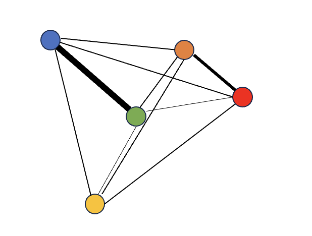
In order to perform clustering, we need to compute the neighborhood graph using and embed the graph in UMAP (Uniform Manifold Approximation and Projection) dimensions. Neighborhood graphs are first determined where nodes represent cells and lines indicate degrees of similarity between cells ie lines with greater weight indicate cells are more closely similar to each other.
graph example
Knowing this, we then embed the graph in UMAP dimensions. UMAP is another dimension reduction technique but is based on the idea that most high dimensional data lies in manifolds. We won’t go into much detail here regarding UMAP, but the below links are helpful to learn more:
# calculate neighborhood graph pp = preprocessing using the first 40 PCssc.pp.neighbors(adata, n_neighbors=10, n_pcs=40)# initial clustering...this part isn't in the official demo but I think they forgot this partsc.tl.leiden(adata)# remedy disconnected clusters...sc.tl.paga(adata) # maps "coarse-grained connectivity structures of complex manifolds", tl = toolkit, paga = partition-based graph abstractionsc.pl.paga(adata, plot=False) # compute the course grained layout, pl = plotsc.tl.umap(adata, init_pos='paga') # embed in umap# embedding of neighborhood graph using UMAPsc.tl.umap(adata)sc.pl.umap(adata, color=['CST3', 'NKG7', 'PPBP'])
---------------------------------------------------------------------------NameError Traceback (most recent call last)
CellIn[13], line 2 1# calculate neighborhood graph pp = preprocessing using the first 40 PCs----> 2sc.pp.neighbors(adata, n_neighbors=10, n_pcs=40)
4# initial clustering...this part isn't in the official demo but I think they forgot this part 5 sc.tl.leiden(adata)
NameError: name 'sc' is not defined
Now, we can finally cluster the data using the Leiden graph-clustering method, which tries to detect communities of nodes.
Again, we won’t go into too much detail regarding this methods, but the below are helpful:
---------------------------------------------------------------------------NameError Traceback (most recent call last)
CellIn[14], line 1----> 1sc.tl.leiden(adata)
2 sc.pl.umap(adata, color=['leiden', 'CST3', 'NKG7'])
NameError: name 'sc' is not defined
In-class exercises
In-class exercise 1: From the AnnData section…instead of creating a csr_matrix can we create a pandas dataframe instead to look at the data more easily?