# First, we'll make a vector to play with
names <- c("rosalind", "marie", "barbara")Data Wrangling Basics
Data Wrangling Day 1
What is data wrangling?
Data wrangling, manipulation, or cleaning is the process of transforming data into a format that is more suitable for analysis. This can include removing missing values, changing the format of data, or combining multiple datasets.
There’s rarely a single way to approach any given data-wrangling problem! Expanding your “toolkit” allows you to tackle problems from different angles.
Objectives of Data Wrangling: Class 1
Be comfortable subsetting vectors and dataframes using both base R and tidyverse functions
Understand what tidy data is and what it looks like
Understand piping basics:
mutate(),filter(),group_by(), andsummarize()
Measure twice, cut once
Before you begin wrangling data, you should be able to:
Define how you want the data to look and why
Document it well so that others (and future you!) know what you did
Know what tools you have and how to use them
Building a toolkit
Working with vectors
Pulling out specific parts of a data set is important when analyzing with R. Indexing, or accessing elements, subsets data based on numeric positions in a vector. You may remember this from the first class. Some things to be aware of when indexing:
Indexing uses brackets. i.e. the 5th element in a vector will be returned if you run
vector[5].It’s helpful for getting several elements at once, or reordering data.
Here are some examples:
# if we print the output, we'd get:
names
[1] "rosalind" "marie" "barbara" # If we want to access the first name, we can use brackets and the position of the name in the vector:
names[1][1] "rosalind"# This works with any position, for example the third name:
names[3][1] "barbara"# You can index more than one position at a time too:
names[c(1,2)][1] "rosalind" "marie" # Changing the order of numbers you supply changes the order of names returned
names[c(2,1)][1] "marie" "rosalind"Working with data frames
This works for two-dimensional structures too, like data frames and matrices. We’d just format it as: dataframe[row,column]. Let’s try it out:
# Make a data frame
df <- data.frame(
  name = c("Rosalind Franklin", "Marie Curie", "Barbara McClintock", "Ada Lovelace", "Dorothy Hodgkin",
           "Lise Meitner", "Grace Hopper", "Chien-Shiung Wu", "Gerty Cori", "Katherine Johnson"),
  field = c("DNA X-ray crystallography", "Radioactivity", "Genetics", "Computer Programming", "X-ray Crystallography",
            "Nuclear Physics", "Computer Programming", "Experimental Physics", "Biochemistry", "Orbital Mechanics"),
  school = c("Cambridge", "Sorbonne", "Cornell", "University of London", "Oxford",
             "University of Berlin", "Yale", "Princeton", "Washington University", "West Virginia University"),
  date_of_birth = c("1920-07-25", "1867-11-07", "1902-06-16", "1815-12-10", "1910-05-12",
                    "1878-11-07", "1906-12-09", "1912-05-31", "1896-08-15", "1918-08-26"),
  working_region = c("Western Europe", "Western Europe", "North America", "Western Europe", "Western Europe", "Western Europe", "North America", "North America", "North America",  "North America")
)

# To get the first row:
df[1,]
name field school date_of_birth
1 Rosalind Franklin DNA X-ray crystallography Cambridge 1920-07-25
working_region
1 Western Europe# or the first column:
df[,1] [1] "Rosalind Franklin" "Marie Curie" "Barbara McClintock"
[4] "Ada Lovelace" "Dorothy Hodgkin" "Lise Meitner"
[7] "Grace Hopper" "Chien-Shiung Wu" "Gerty Cori"
[10] "Katherine Johnson" # for specific cells:
df[2,3][1] "Sorbonne"# We can use the column name instead of numbers:
df[2,"school"][1] "Sorbonne"# We can do the same thing by using a dollar sign:
df$name [1] "Rosalind Franklin" "Marie Curie" "Barbara McClintock"
[4] "Ada Lovelace" "Dorothy Hodgkin" "Lise Meitner"
[7] "Grace Hopper" "Chien-Shiung Wu" "Gerty Cori"
[10] "Katherine Johnson" # We can also give a list of columns
# which return in the order provided
df[,c("school","name")] school name
1 Cambridge Rosalind Franklin
2 Sorbonne Marie Curie
3 Cornell Barbara McClintock
4 University of London Ada Lovelace
5 Oxford Dorothy Hodgkin
6 University of Berlin Lise Meitner
7 Yale Grace Hopper
8 Princeton Chien-Shiung Wu
9 Washington University Gerty Cori
10 West Virginia University Katherine JohnsonStandard data formats and Tidy
That data, and most two-dimensional data sets (data frames, matrices, etc.) is often organized the similarly:
Each variable is its own column
Each observation is its own row
Each value is a single cell.
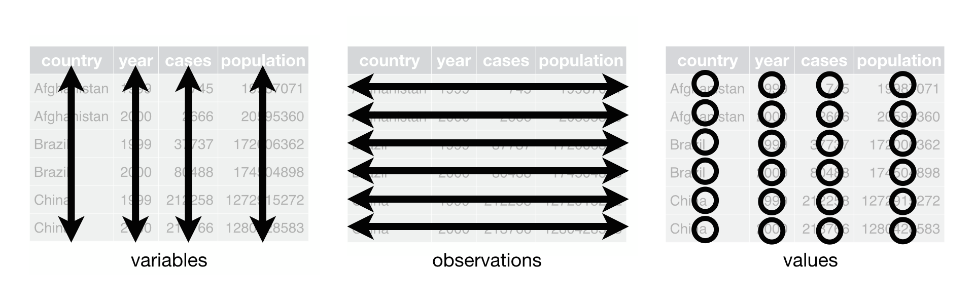
This follows the tidy data style, an approach to handling data in R that aims to be clear and readable.
Tidiest Universe
The bundle of tidy-associated packages is called the tidyverse, and it’s a 🔥 hot-topic 🔥 in the R world. In fact, ggplot is a package that you have already used that is part of the tidyverse! Most data wrangling problems can be solved with tidy or base (default) R functions. This can lead to some headaches for beginners, as there are multiple ways to accomplish the same thing!
Review the below datasets. Given the above criteria, are they tidy? If not, write out in words what you would need to do. The first one is done as an example.
library(tidyverse)
head(relig_income)
# A tibble: 6 × 11
religion `<$10k` `$10-20k` `$20-30k` `$30-40k` `$40-50k` `$50-75k` `$75-100k`
<chr> <dbl> <dbl> <dbl> <dbl> <dbl> <dbl> <dbl>
1 Agnostic 27 34 60 81 76 137 122
2 Atheist 12 27 37 52 35 70 73
3 Buddhist 27 21 30 34 33 58 62
4 Catholic 418 617 732 670 638 1116 949
5 Don’t kn… 15 14 15 11 10 35 21
6 Evangeli… 575 869 1064 982 881 1486 949
# ℹ 3 more variables: `$100-150k` <dbl>, `>150k` <dbl>,
# `Don't know/refused` <dbl>This data is not tidy because there are variables (income) in the columns. A tidy dataset would have three columns: religion, income, and number of respondents (n). We would need to pivot the data to create new columns called income and n.
head(billboard)# A tibble: 6 × 79
artist track date.entered wk1 wk2 wk3 wk4 wk5 wk6 wk7 wk8
<chr> <chr> <date> <dbl> <dbl> <dbl> <dbl> <dbl> <dbl> <dbl> <dbl>
1 2 Pac Baby… 2000-02-26 87 82 72 77 87 94 99 NA
2 2Ge+her The … 2000-09-02 91 87 92 NA NA NA NA NA
3 3 Doors Do… Kryp… 2000-04-08 81 70 68 67 66 57 54 53
4 3 Doors Do… Loser 2000-10-21 76 76 72 69 67 65 55 59
5 504 Boyz Wobb… 2000-04-15 57 34 25 17 17 31 36 49
6 98^0 Give… 2000-08-19 51 39 34 26 26 19 2 2
# ℹ 68 more variables: wk9 <dbl>, wk10 <dbl>, wk11 <dbl>, wk12 <dbl>,
# wk13 <dbl>, wk14 <dbl>, wk15 <dbl>, wk16 <dbl>, wk17 <dbl>, wk18 <dbl>,
# wk19 <dbl>, wk20 <dbl>, wk21 <dbl>, wk22 <dbl>, wk23 <dbl>, wk24 <dbl>,
# wk25 <dbl>, wk26 <dbl>, wk27 <dbl>, wk28 <dbl>, wk29 <dbl>, wk30 <dbl>,
# wk31 <dbl>, wk32 <dbl>, wk33 <dbl>, wk34 <dbl>, wk35 <dbl>, wk36 <dbl>,
# wk37 <dbl>, wk38 <dbl>, wk39 <dbl>, wk40 <dbl>, wk41 <dbl>, wk42 <dbl>,
# wk43 <dbl>, wk44 <dbl>, wk45 <dbl>, wk46 <dbl>, wk47 <dbl>, wk48 <dbl>, …dplyr verbs
One of the most popular tidyverse packages, dplyr, offers a suite of helpful and readable functions for data manipulation. Let’s get started with how it can help you see your data:
- The library is already synchronized with the lockfile.dplyr::glimpse(df)Rows: 10
Columns: 5
$ name <chr> "Rosalind Franklin", "Marie Curie", "Barbara McClintock…
$ field <chr> "DNA X-ray crystallography", "Radioactivity", "Genetics…
$ school <chr> "Cambridge", "Sorbonne", "Cornell", "University of Lond…
$ date_of_birth <chr> "1920-07-25", "1867-11-07", "1902-06-16", "1815-12-10",…
$ working_region <chr> "Western Europe", "Western Europe", "North America", "W…With the glimpse function we see that this is a data frame with 3 observations and 3 variables. We can also see the type of each variable and the first few values.
Tip
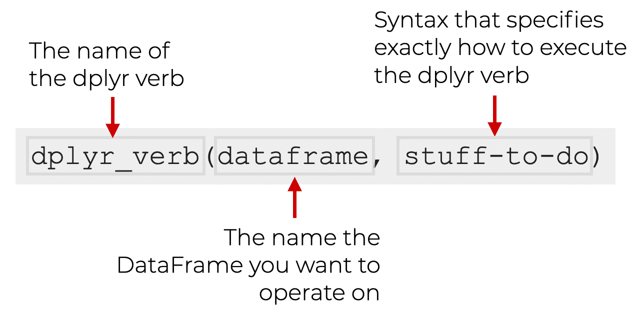
dplyr functions have a lot in common:
The first argument is always a data frame
The following arguments typically specify which columns to operate on, using the variable names (without quotes)
The output is always a new data frame
The dplyr package has a set of functions that are used to manipulate data frames (you may see these referred to as “verbs”, and it may also be helpful to think of them as verbs performing an action on your dataframe). These functions can either act on rows (e.g. filter out specific rows by some condition) or columns (e.g. select columns XYZ). There are also functions for working with groups (e.g. group rows by what values they have in a column with group_by).
The most important verbs that operate on rows of a dataset are filter(), which changes which rows are present without changing their order, and arrange(), which changes the order of the rows without changing which are present. Both functions only affect the rows, and the columns are left unchanged. We’ll also discuss distinct() which finds rows with unique values but unlike arrange() and filter() it can also optionally modify the columns.
More information about functions like this can be found here.
There are four important verbs that affect the columns without changing the rows: mutate() creates new columns that are derived from the existing columns, select() changes which columns are present, rename() changes the names of the columns, and relocate() changes the positions of the columns.
More information about functions like this can be found here.
group_by allows you to create groups using more than one variable.
summarize works on grouped objects and allows you to calculate a single summary statistic, reducing the data frame to have a single row for each group.
The slice family of functions allows you to extract specific rows within each group
More information about functions like this can be found here.
Tip
dplyr verbs work great as a team!
Although these were basic examples, hopefully you feel a little more confident about working with vectors, and data frames using dplyr verbs to clean and manipulate data. Give some of them a try with the billboard dataset below. Happy Wrangling!
# First, let's make this data set tidy :)
billboard2 <- billboard |>
  pivot_longer(
    wk1:wk76,
    names_to = "week",
    values_to = "rank",
    values_drop_na = TRUE
)- Use
mutate()to add a new column calledweek_numberthat is the week as integer (i.e. wk1 is 1) - Use
filter()to get all the songs by Eve. - Use
mutate()to add a new column calledyearwith the year derived from the date in the columndate.entered
Functions on functions
An introduction to pipes
Data scientists often want to make many changes to their data at one time. Typically, this means using more than one function at once. However, the way we’ve been writing our scripts so far would make for some very confusing looking code.
For example, let’s use dplyr functions to perform two operations on our data set of scientists: filter for those born after 1900 and then arrange them by date of birth.
Here we first filter and then arrange. Note that we are creating an intermediate variable in between the steps.
# Filtering for scientists born after 1900
filtered_data <- filter(df, as.Date(date_of_birth) > as.Date("1900-01-01"))

# Arranging the filtered data by date of birth
arranged_data <- arrange(filtered_data, date_of_birth)
We can do the same thing without creating an intermediate variable. It’s more compact but can start to get confusing if we add more functions.
arranged_data <- arrange(filter(df, as.Date(date_of_birth) > as.Date("1900-01-01")), date_of_birth)The pipe operator, |>, is a tool that can help make the script more readable. It allows us to pass the result of one function directly into the next. Think of it as saying, “and then..”
Let’s dissect our goal: filter for those born after 1900 and then arrange them by date of birth.
filter is doing the filter for… part
arrange is doing the arrange them… part
and the pipe, |>, is going to do the and then… part.
# Using pipes
arranged_data <- df |>
  filter(as.Date(date_of_birth) > as.Date("1900-01-01")) |>
  arrange(date_of_birth)
Once you’re comfortable with this style, you should be able to read it as: Take data and then filter by DoB and then arrange by DoB. This helps keep our code both clean and readable.
Tip
There are two pipe operators: |> and %>%. They work almost the exact same way. %>% is from the magrittr package and was the only way to pipe before version R 4.1.0. You may see %>%more frequently in code from previous lab members.
Placeholders
The Placeholder operator allows more control over where the LHS (left hand side) is placed into the RHS (right hand side) of the pipe operator.
%>% uses . as its placeholder operator. In addition to this, you may use . multiple times on the RHS
3 %>% head(x = letters, n = .)[1] "a" "b" "c"3 %>% sum(2, ., .)[1] 8|> uses _ as its placeholder operator. However, the _ placeholder must only be used once and the argument must be named
3 |> head(x = letters, n = _)[1] "a" "b" "c"#3 |> sum(2, _)#| #| #| #| #add3 <- function(x, y, z) x + y + z
#3 |> add3(2, y = _, z = _)
Right Hand Side (RHS)
%>% can take a function name on the RHS
letters %>% head[1] "a" "b" "c" "d" "e" "f"The RHS for |> must be a function with ()
#letters |> headletters |> head()[1] "a" "b" "c" "d" "e" "f"
Anonymous Functions
%>% can take expressions in curly braces {}
x <- 10
5 %>% {x + .}
[1] 15|> must have a function call on RHS
#x <- 10
#5 |> {x + _}
5 |> {function(y) x + y}()[1] 15To summarize, %>% is slightly more lenient than |> when it comes to the Placeholder operator, the Right Hand Side (RHS) and Anonymous functions.
Using the same billboard2 dataset from above, try out using pipes on the following:
- Use
filter(),group_by(),and aslicefunction (read the documentation linked above to determine which one!) to create a new dataframe callednumber_one_hits_2000that has the top ranked song for each week from the year 2000.
- Use some of the same functions to create a new dataframe called
number_one_hitsthat has the top ranked song for each week from each year. - What was the highest ranking Creed’s “Higher” achieved?
- Using
group_by()andsummarize()how many unique songs did Whitney Houston have on the charts?