R Coding Basics
Coding Basics, Day 1
Introduction
Many biologists starting out in bioinformatics tend to equate “learning bioinformatics” with “learning how to run bioinformatics software”… This is analogous to thinking “learning molecular biology” is just “learning pipetting.”
— Vince Buffalo
In Vince’s quote above, replace “bioinformatics” with “coding.”
Our goal for How to Learn to Code is to familiarize students with the R programming language and RStudio environment, equip students with the skills and knowledge to wrangle, visualize, and analyze data, and to provide a foundation for more advanced coding skills.
In Module 1: Coding Basics, we will cover:
- Variables
- Reproducible environments
- RStudio IDE
- Various R script and file formats
- R syntax
- Commenting, writing, and executing code
- Functions
- Data structures in R
- Data types in R
- Manipulating data types and structures
Curious about what the rest of the classes will look like?
Module 1: Coding Basics
Module 2: Data Visualization
Module 3: Data Wrangling
Module 4: Putting it all together: Projects
Objectives of Coding Basics: Class 1
Be able to create a variable, define what it is, and follow good variable naming practices
Understand basic data structures in R
Understand basic data types in R
Perform basic manipulations with data structures and types
Describe benefits of knowing how to code
Exploring a dataset
R has a few built in datasets that we can use until we cover installing/loading packages and reading in data files. For the following examples we will use a built-in dataset in R called “iris” that has some measurements across a few species of flowers. It is one of the most popular built-in datasets in R. We will use this dataset to explore key coding concepts: variables, data types, and functions.
First, let’s take a look at the dataset. You can view the dataset multiple ways. Let’s try one–copy the below line of code into your console and run it.
irisAs we can see, this dataset has a few columns of numbers, in addition to the species. Let’s try a few other ways to look at this dataset. As you try each method, think about what is different about each method. When would one method be more beneficial than another?
head(iris) Sepal.Length Sepal.Width Petal.Length Petal.Width Species
1 5.1 3.5 1.4 0.2 setosa
2 4.9 3.0 1.4 0.2 setosa
3 4.7 3.2 1.3 0.2 setosa
4 4.6 3.1 1.5 0.2 setosa
5 5.0 3.6 1.4 0.2 setosa
6 5.4 3.9 1.7 0.4 setosa#View(iris)You are probably already thinking of questions you need the answers to in order to familiarize yourself with this dataset. What does each row represent? Each column? How many observations (rows) do we have? What is the average petal length? Think about other questions you may want to ask. Think about how you would go about answering those questions with what you already know. Maybe you’d count each row on your screen to get the number of observations, or copy the values under Petal.Length into your phone calculator to calculate the mean. By the end of this class, you’ll be able to do all those things very quickly in R!
Variables
A variable is a named space in your computer’s memory which can be referenced and manipulated. It’s sort of a name you give “something”, and that something can be just about anything.
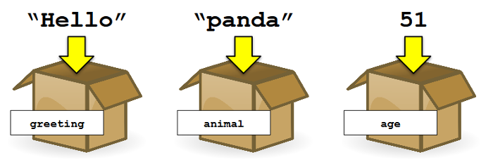
Variables in R are created (assigned) using an arrow: <- The variable name always goes on the left, and the thing being assigned to that variable on the right. For example:
greeting <- "Hello"
animal <- "panda"
age <- 51
The value something is assigned to is often referred to as the variable name. For example, the variable name of "Hello" is greeting . We used really basic variable names–just letters, that are real words, all lowercase. Of course, there are other ways to name variables too! Play around with variable names. Try using uppercase letters, symbols, and numbers. What works, and what doesn’t? Come up with some rules for variable naming. Here’s some variable naming ideas to get you started:
GrEeTiNg <- "Hello"
5greeting <- "Hello"
greeting.5 <- "Hello"
greeting@5 <- "Hello"
Now that you know some general rules for variable naming, we can refer to the Style Guide for “proper” variable/object naming. Update your variable naming rule to include the preferred style for variable names according to the Style Guide.
And now that we know how to properly name variables, assign the iris dataset to a variable!
iris_dataset_copy <- irisData types
As you probably know from your own work, data can come in many forms. You can classify dragons as either “purple” or “green” and also record the number of spines on their backs as numeric types (15, 27). Data types are important to understand in R because the type of data impacts what you can do with it. For example, it wouldn’t make sense to calculate a mean for the dragon color, but it would for the number of back spines.
In R, we will focus on three basic data types that are used specify the type of data stored in a variable (there are a few more, but you probably won’t ever run into them): character, numeric, and logical.
Character: A character represents a string value. This can be anything from a single letter to entire paragraphs. Examples include "a", "B", "c is third", "5"
Numeric: A decimal value. Examples include 1.0, 3.1415926535.
Logical: Logical data types have only two possible values: TRUE or FALSE.
So far, we have learned about basic data structures (vectors, matrices, etc.) and basic data types (numeric, character, logical). Now, we want to start manipulating or doing things to them that can be helpful.
Converting Data Types
For example, sometimes when we read in data from a file, numbers can appear as strings of characters rather than a “numeric” type.
my_numbers <- c("4", "2", "7", "10")
print(my_numbers)
[1] "4" "2" "7" "10"How can we tell? Because the numbers above are in quotations, indicating that they are of the character type and R is interpreting them as text. Before doing any math or further analysis with these data points, it’s a good idea to convert them to the numeric type first.
my_numbers <- as.numeric(my_numbers)
print(my_numbers)
[1] 4 2 7 10Note that the quotations are now gone. Now, we can do basic (or more advanced) calculations like the ones below.
# Get minimum out of a list of values
min(my_numbers)
[1] 2# Get maximum out of a list of values
max(my_numbers)[1] 10# Get average (mean) out of a list of values
mean(my_numbers)[1] 5.75We can also sort this list of values to go from smallest to largest. After doing so, the smallest value will be first in the list and the largest value will be last.
my_numbers <- sort(my_numbers)
my_numbers
[1] 2 4 7 10We can reverse the order to go from largest to smallest. There is an option using the sort function to do this.
my_numbers <- sort(my_numbers, decreasing = TRUE)
my_numbers
[1] 10 7 4 2Accessing parts of a list
One thing we’ll be doing a lot of is looking at parts of our data. For example, we might want to look at individual items in a vector. These items could be numbers or characters.
my_data <- c("A", "B", "C", "D", "E", "F")
my_data
[1] "A" "B" "C" "D" "E" "F"In this case, let’s say I’m really interested in that “E” and want to pull it out separately from the rest of the data. I can do that with “indexing”. Here, I can tell that it’s the 5th item in the list, so I can extract it using the following:
my_data[5][1] "E"We can also extract multiple items. If we wanted “D”, “E”, and “F”, we can get all the values from item 4 (“D”) to item 6 (“F”).
my_data[4:6][1] "D" "E" "F"Let’s say we forgot to include some of our data and now we want to add it to this list. We can update my_data to also include these values.
my_data <- c(my_data, "G", "H", "I")
my_data
[1] "A" "B" "C" "D" "E" "F" "G" "H" "I"Before we move on, let’s cover creating vectors. We already did this several times above, but didn’t discuss it. Typically, we’ll want to make vectors of numbers (e.g. our data values) or vectors of characters (e.g. labels for our data). Depending on whether we use quotes or not, R will interpret them as either numeric vectors or character vectors.
# Numeric vector
numeric_vector <- c(1, 2, 3, 4, 5)
numeric_vector
[1] 1 2 3 4 5# Character vector
character_vector <- c("apple", "banana", "orange")
character_vector[1] "apple" "banana" "orange"Remember the iris dataset from earlier? Let’s return to it to cover extracting some of the rows or columns from this data.
We can access specific columns in one of two ways. Typically, we will want to access it by the name of the column. We do this using the name of the data frame, followed by the dollar sign, and finally the name of the column. For example:
iris$Petal.Length [1] 1.4 1.4 1.3 1.5 1.4 1.7 1.4 1.5 1.4 1.5 1.5 1.6 1.4 1.1 1.2 1.5 1.3 1.4
[19] 1.7 1.5 1.7 1.5 1.0 1.7 1.9 1.6 1.6 1.5 1.4 1.6 1.6 1.5 1.5 1.4 1.5 1.2
[37] 1.3 1.4 1.3 1.5 1.3 1.3 1.3 1.6 1.9 1.4 1.6 1.4 1.5 1.4 4.7 4.5 4.9 4.0
[55] 4.6 4.5 4.7 3.3 4.6 3.9 3.5 4.2 4.0 4.7 3.6 4.4 4.5 4.1 4.5 3.9 4.8 4.0
[73] 4.9 4.7 4.3 4.4 4.8 5.0 4.5 3.5 3.8 3.7 3.9 5.1 4.5 4.5 4.7 4.4 4.1 4.0
[91] 4.4 4.6 4.0 3.3 4.2 4.2 4.2 4.3 3.0 4.1 6.0 5.1 5.9 5.6 5.8 6.6 4.5 6.3
[109] 5.8 6.1 5.1 5.3 5.5 5.0 5.1 5.3 5.5 6.7 6.9 5.0 5.7 4.9 6.7 4.9 5.7 6.0
[127] 4.8 4.9 5.6 5.8 6.1 6.4 5.6 5.1 5.6 6.1 5.6 5.5 4.8 5.4 5.6 5.1 5.1 5.9
[145] 5.7 5.2 5.0 5.2 5.4 5.1If we knew which column it was (or it wasn’t named), we can also use indexing. Inside the brackets, we will need to indicate which [row , column] we want from this data frame. Since we want all the rows, we will leave the “row” blank. We can see that the Petal.Length was the 3rd column.
iris[, 3] [1] 1.4 1.4 1.3 1.5 1.4 1.7 1.4 1.5 1.4 1.5 1.5 1.6 1.4 1.1 1.2 1.5 1.3 1.4
[19] 1.7 1.5 1.7 1.5 1.0 1.7 1.9 1.6 1.6 1.5 1.4 1.6 1.6 1.5 1.5 1.4 1.5 1.2
[37] 1.3 1.4 1.3 1.5 1.3 1.3 1.3 1.6 1.9 1.4 1.6 1.4 1.5 1.4 4.7 4.5 4.9 4.0
[55] 4.6 4.5 4.7 3.3 4.6 3.9 3.5 4.2 4.0 4.7 3.6 4.4 4.5 4.1 4.5 3.9 4.8 4.0
[73] 4.9 4.7 4.3 4.4 4.8 5.0 4.5 3.5 3.8 3.7 3.9 5.1 4.5 4.5 4.7 4.4 4.1 4.0
[91] 4.4 4.6 4.0 3.3 4.2 4.2 4.2 4.3 3.0 4.1 6.0 5.1 5.9 5.6 5.8 6.6 4.5 6.3
[109] 5.8 6.1 5.1 5.3 5.5 5.0 5.1 5.3 5.5 6.7 6.9 5.0 5.7 4.9 6.7 4.9 5.7 6.0
[127] 4.8 4.9 5.6 5.8 6.1 6.4 5.6 5.1 5.6 6.1 5.6 5.5 4.8 5.4 5.6 5.1 5.1 5.9
[145] 5.7 5.2 5.0 5.2 5.4 5.1Let’s say we didn’t care the exact measurement of the Petal.Length of these flowers. We only cared whether they were “big” or not, and let’s say that “big” is a Petal.Length of greater than 5.
iris$Petal.Length > 5 [1] FALSE FALSE FALSE FALSE FALSE FALSE FALSE FALSE FALSE FALSE FALSE FALSE
[13] FALSE FALSE FALSE FALSE FALSE FALSE FALSE FALSE FALSE FALSE FALSE FALSE
[25] FALSE FALSE FALSE FALSE FALSE FALSE FALSE FALSE FALSE FALSE FALSE FALSE
[37] FALSE FALSE FALSE FALSE FALSE FALSE FALSE FALSE FALSE FALSE FALSE FALSE
[49] FALSE FALSE FALSE FALSE FALSE FALSE FALSE FALSE FALSE FALSE FALSE FALSE
[61] FALSE FALSE FALSE FALSE FALSE FALSE FALSE FALSE FALSE FALSE FALSE FALSE
[73] FALSE FALSE FALSE FALSE FALSE FALSE FALSE FALSE FALSE FALSE FALSE TRUE
[85] FALSE FALSE FALSE FALSE FALSE FALSE FALSE FALSE FALSE FALSE FALSE FALSE
[97] FALSE FALSE FALSE FALSE TRUE TRUE TRUE TRUE TRUE TRUE FALSE TRUE
[109] TRUE TRUE TRUE TRUE TRUE FALSE TRUE TRUE TRUE TRUE TRUE FALSE
[121] TRUE FALSE TRUE FALSE TRUE TRUE FALSE FALSE TRUE TRUE TRUE TRUE
[133] TRUE TRUE TRUE TRUE TRUE TRUE FALSE TRUE TRUE TRUE TRUE TRUE
[145] TRUE TRUE FALSE TRUE TRUE TRUESome of them are “big” (with values of TRUE) and many of them are “small” (with values of FALSE). We can add this information to our dataset by making another column. Similar to how we extracted this column, we can also make a new one (with a name of our choice).
iris$BigPetals <- iris$Petal.Length > 5And now it is added to our dataset.
iris Sepal.Length Sepal.Width Petal.Length Petal.Width Species BigPetals
1 5.1 3.5 1.4 0.2 setosa FALSE
2 4.9 3.0 1.4 0.2 setosa FALSE
3 4.7 3.2 1.3 0.2 setosa FALSE
4 4.6 3.1 1.5 0.2 setosa FALSE
5 5.0 3.6 1.4 0.2 setosa FALSE
6 5.4 3.9 1.7 0.4 setosa FALSE
7 4.6 3.4 1.4 0.3 setosa FALSE
8 5.0 3.4 1.5 0.2 setosa FALSE
9 4.4 2.9 1.4 0.2 setosa FALSE
10 4.9 3.1 1.5 0.1 setosa FALSE
11 5.4 3.7 1.5 0.2 setosa FALSE
12 4.8 3.4 1.6 0.2 setosa FALSE
13 4.8 3.0 1.4 0.1 setosa FALSE
14 4.3 3.0 1.1 0.1 setosa FALSE
15 5.8 4.0 1.2 0.2 setosa FALSE
16 5.7 4.4 1.5 0.4 setosa FALSE
17 5.4 3.9 1.3 0.4 setosa FALSE
18 5.1 3.5 1.4 0.3 setosa FALSE
19 5.7 3.8 1.7 0.3 setosa FALSE
20 5.1 3.8 1.5 0.3 setosa FALSE
21 5.4 3.4 1.7 0.2 setosa FALSE
22 5.1 3.7 1.5 0.4 setosa FALSE
23 4.6 3.6 1.0 0.2 setosa FALSE
24 5.1 3.3 1.7 0.5 setosa FALSE
25 4.8 3.4 1.9 0.2 setosa FALSE
26 5.0 3.0 1.6 0.2 setosa FALSE
27 5.0 3.4 1.6 0.4 setosa FALSE
28 5.2 3.5 1.5 0.2 setosa FALSE
29 5.2 3.4 1.4 0.2 setosa FALSE
30 4.7 3.2 1.6 0.2 setosa FALSE
31 4.8 3.1 1.6 0.2 setosa FALSE
32 5.4 3.4 1.5 0.4 setosa FALSE
33 5.2 4.1 1.5 0.1 setosa FALSE
34 5.5 4.2 1.4 0.2 setosa FALSE
35 4.9 3.1 1.5 0.2 setosa FALSE
36 5.0 3.2 1.2 0.2 setosa FALSE
37 5.5 3.5 1.3 0.2 setosa FALSE
38 4.9 3.6 1.4 0.1 setosa FALSE
39 4.4 3.0 1.3 0.2 setosa FALSE
40 5.1 3.4 1.5 0.2 setosa FALSE
41 5.0 3.5 1.3 0.3 setosa FALSE
42 4.5 2.3 1.3 0.3 setosa FALSE
43 4.4 3.2 1.3 0.2 setosa FALSE
44 5.0 3.5 1.6 0.6 setosa FALSE
45 5.1 3.8 1.9 0.4 setosa FALSE
46 4.8 3.0 1.4 0.3 setosa FALSE
47 5.1 3.8 1.6 0.2 setosa FALSE
48 4.6 3.2 1.4 0.2 setosa FALSE
49 5.3 3.7 1.5 0.2 setosa FALSE
50 5.0 3.3 1.4 0.2 setosa FALSE
51 7.0 3.2 4.7 1.4 versicolor FALSE
52 6.4 3.2 4.5 1.5 versicolor FALSE
53 6.9 3.1 4.9 1.5 versicolor FALSE
54 5.5 2.3 4.0 1.3 versicolor FALSE
55 6.5 2.8 4.6 1.5 versicolor FALSE
56 5.7 2.8 4.5 1.3 versicolor FALSE
57 6.3 3.3 4.7 1.6 versicolor FALSE
58 4.9 2.4 3.3 1.0 versicolor FALSE
59 6.6 2.9 4.6 1.3 versicolor FALSE
60 5.2 2.7 3.9 1.4 versicolor FALSE
61 5.0 2.0 3.5 1.0 versicolor FALSE
62 5.9 3.0 4.2 1.5 versicolor FALSE
63 6.0 2.2 4.0 1.0 versicolor FALSE
64 6.1 2.9 4.7 1.4 versicolor FALSE
65 5.6 2.9 3.6 1.3 versicolor FALSE
66 6.7 3.1 4.4 1.4 versicolor FALSE
67 5.6 3.0 4.5 1.5 versicolor FALSE
68 5.8 2.7 4.1 1.0 versicolor FALSE
69 6.2 2.2 4.5 1.5 versicolor FALSE
70 5.6 2.5 3.9 1.1 versicolor FALSE
71 5.9 3.2 4.8 1.8 versicolor FALSE
72 6.1 2.8 4.0 1.3 versicolor FALSE
73 6.3 2.5 4.9 1.5 versicolor FALSE
74 6.1 2.8 4.7 1.2 versicolor FALSE
75 6.4 2.9 4.3 1.3 versicolor FALSE
76 6.6 3.0 4.4 1.4 versicolor FALSE
77 6.8 2.8 4.8 1.4 versicolor FALSE
78 6.7 3.0 5.0 1.7 versicolor FALSE
79 6.0 2.9 4.5 1.5 versicolor FALSE
80 5.7 2.6 3.5 1.0 versicolor FALSE
81 5.5 2.4 3.8 1.1 versicolor FALSE
82 5.5 2.4 3.7 1.0 versicolor FALSE
83 5.8 2.7 3.9 1.2 versicolor FALSE
84 6.0 2.7 5.1 1.6 versicolor TRUE
85 5.4 3.0 4.5 1.5 versicolor FALSE
86 6.0 3.4 4.5 1.6 versicolor FALSE
87 6.7 3.1 4.7 1.5 versicolor FALSE
88 6.3 2.3 4.4 1.3 versicolor FALSE
89 5.6 3.0 4.1 1.3 versicolor FALSE
90 5.5 2.5 4.0 1.3 versicolor FALSE
91 5.5 2.6 4.4 1.2 versicolor FALSE
92 6.1 3.0 4.6 1.4 versicolor FALSE
93 5.8 2.6 4.0 1.2 versicolor FALSE
94 5.0 2.3 3.3 1.0 versicolor FALSE
95 5.6 2.7 4.2 1.3 versicolor FALSE
96 5.7 3.0 4.2 1.2 versicolor FALSE
97 5.7 2.9 4.2 1.3 versicolor FALSE
98 6.2 2.9 4.3 1.3 versicolor FALSE
99 5.1 2.5 3.0 1.1 versicolor FALSE
100 5.7 2.8 4.1 1.3 versicolor FALSE
101 6.3 3.3 6.0 2.5 virginica TRUE
102 5.8 2.7 5.1 1.9 virginica TRUE
103 7.1 3.0 5.9 2.1 virginica TRUE
104 6.3 2.9 5.6 1.8 virginica TRUE
105 6.5 3.0 5.8 2.2 virginica TRUE
106 7.6 3.0 6.6 2.1 virginica TRUE
107 4.9 2.5 4.5 1.7 virginica FALSE
108 7.3 2.9 6.3 1.8 virginica TRUE
109 6.7 2.5 5.8 1.8 virginica TRUE
110 7.2 3.6 6.1 2.5 virginica TRUE
111 6.5 3.2 5.1 2.0 virginica TRUE
112 6.4 2.7 5.3 1.9 virginica TRUE
113 6.8 3.0 5.5 2.1 virginica TRUE
114 5.7 2.5 5.0 2.0 virginica FALSE
115 5.8 2.8 5.1 2.4 virginica TRUE
116 6.4 3.2 5.3 2.3 virginica TRUE
117 6.5 3.0 5.5 1.8 virginica TRUE
118 7.7 3.8 6.7 2.2 virginica TRUE
119 7.7 2.6 6.9 2.3 virginica TRUE
120 6.0 2.2 5.0 1.5 virginica FALSE
121 6.9 3.2 5.7 2.3 virginica TRUE
122 5.6 2.8 4.9 2.0 virginica FALSE
123 7.7 2.8 6.7 2.0 virginica TRUE
124 6.3 2.7 4.9 1.8 virginica FALSE
125 6.7 3.3 5.7 2.1 virginica TRUE
126 7.2 3.2 6.0 1.8 virginica TRUE
127 6.2 2.8 4.8 1.8 virginica FALSE
128 6.1 3.0 4.9 1.8 virginica FALSE
129 6.4 2.8 5.6 2.1 virginica TRUE
130 7.2 3.0 5.8 1.6 virginica TRUE
131 7.4 2.8 6.1 1.9 virginica TRUE
132 7.9 3.8 6.4 2.0 virginica TRUE
133 6.4 2.8 5.6 2.2 virginica TRUE
134 6.3 2.8 5.1 1.5 virginica TRUE
135 6.1 2.6 5.6 1.4 virginica TRUE
136 7.7 3.0 6.1 2.3 virginica TRUE
137 6.3 3.4 5.6 2.4 virginica TRUE
138 6.4 3.1 5.5 1.8 virginica TRUE
139 6.0 3.0 4.8 1.8 virginica FALSE
140 6.9 3.1 5.4 2.1 virginica TRUE
141 6.7 3.1 5.6 2.4 virginica TRUE
142 6.9 3.1 5.1 2.3 virginica TRUE
143 5.8 2.7 5.1 1.9 virginica TRUE
144 6.8 3.2 5.9 2.3 virginica TRUE
145 6.7 3.3 5.7 2.5 virginica TRUE
146 6.7 3.0 5.2 2.3 virginica TRUE
147 6.3 2.5 5.0 1.9 virginica FALSE
148 6.5 3.0 5.2 2.0 virginica TRUE
149 6.2 3.4 5.4 2.3 virginica TRUE
150 5.9 3.0 5.1 1.8 virginica TRUEFunctions
A function is a block of code that does a task. It only executes that task when it is called/executed. Using a function in R always follows the same basic format:
function_name(arguments)
The arguments are passed to the function, i.e. they are values that the function will manipulate. Functions can be built into R, included in packages, or you can write your own.
Functions can do very basic tasks:
print("Hello world!")[1] "Hello world!"Or more complex tasks, where multiple arguments are required, each separated by a comma:
substr(x = "Hello world!", start = 2, stop = 4)[1] "ell"We have already been using functions throughout this class–some examples include sort(), min(), and max().
We will be using functions all the time in How to Learn to Code, but for today just know what a function is and what an argument is. Whenever you use a function, it’s important to ensure you understand what it’s doing: are you getting the expected result? Are you using the input arguments correctly? That is not only crucial for learning how to code, but how to think like a coder.
I already need help!
Since this is a built-in dataset, we can get some help. Try running the code below:
?iris
?mean()
Adding a ? before the name of a function or data frame (built-in or from a package) pulls up a help file in the Help tab of the Output pane. If you aren’t sure what a function does, this should be your first step.