| update | condition | minimal_avg.fitness | minimal_avg.offspring.cost | minimal_avg.energy.acq.rate | minimal_pop.size | selective_avg.fitness | selective_avg.offspring.cost | selective_avg.energy.acq.rate | selective_pop.size | rich_avg.fitness | rich_avg.offspring.cost | rich_avg.energy.acq.rate | rich_pop.size |
|---|---|---|---|---|---|---|---|---|---|---|---|---|---|
| 0 | wildtype-only | 0.3587786 | 131 | 47 | 1 | 0.2486772 | 189 | 47 | 1 | 0.3587786 | 131 | 47 | 1 |
| 1 | wildtype-only | 0.3587786 | 131 | 47 | 1 | 0.2486772 | 189 | 47 | 1 | 0.3587786 | 131 | 47 | 1 |
| 2 | wildtype-only | 0.3587786 | 131 | 47 | 1 | 0.2486772 | 189 | 47 | 1 | 0.3587786 | 131 | 47 | 1 |
| 3 | wildtype-only | 0.3587786 | 131 | 47 | 1 | 0.2486772 | 189 | 47 | 1 | 0.3587786 | 131 | 47 | 1 |
| 4 | wildtype-only | 0.3587786 | 131 | 47 | 2 | 0.2486772 | 189 | 47 | 1 | 0.3587786 | 131 | 47 | 2 |
| 5 | wildtype-only | 0.3587786 | 131 | 47 | 2 | 0.2486772 | 189 | 47 | 1 | 0.3587786 | 131 | 47 | 2 |
Practicing on Real-World Data
Project Management, Day 2
Final class!
In the previous class, you completed the following steps:
Created a GitHub account.
Linked your GitHub account with your Longleaf account.
Created and pushed your first repository to GitHub.
Today, now that you’ve been through the entire course, we want to reinforce some of the skills that you’ve learned by having you apply your knowledge to several existing datasets and go through the wrangling, analysis, and visualization process as independently as you can. By the end of this lesson, you should have a GitHub repo containing scripts for wrangling and analysis for at least one of these datasets that you can show to others (or at least have as a reference for your future self).
For each of these datasets (or as many as time allows), we’d like you to do some basic analysis, including the following steps:
Create a directory for the analysis of this dataset, using best practices discussed in the previous class.
Load in the data.
Perform some initial data exploration (What are the rows? What are the columns? How many samples does this dataset have? etc.)
Identify at least 1 research question that you could try to answer with this dataset.
Format the data in a way that allows for this analysis.
Visualize the data in helpful ways to answer your question.
Make your code reproducible by using GitHub.
To help with your analyses, we have included a project template document outlining these steps that you are welcome to use in data/project-day-2-files/example-analyses; the location of additional files are specified below.
Datasets
The csvs are available under in data/project-day-2-files/datasets. We have provided links to data that is publicly available for download, as well as some related publications that may give you more information about the data.
These datasets were chosen because we thought they represented a good variety in the different kinds of wrangling and visualization challenges you might encounter with your own data in the future: we have highlighted a few specific R skills that some of these datasets were meant to challenge you on.
Note
The datasets are presented roughly in order of increasing wrangling complexity. Though you should have most of the basic skills you need to wrangle and analyze these datasets, we have specifically provided some code to aid you in certain wrangling tasks for some of the later datasets: see the “Analysis ideas and hints” callout for each dataset.
For each dataset, we have provided a description of the research question/data collection methods, metadata, and the first few lines of each dataset. Read through these descriptions and work on the dataset you find most interesting. Feel free to work with a partner!
But I thought this was HTLTCode, not HTLTScience!
To get the most out of today’s activities, we highly encourage you to practice going through the whole data analysis workflow as independently as you can, using your notes and practicing your Googling skills to develop your own research questions and analysis ideas for these datasets.
That said, we have prepared some example research questions and figures for each dataset to get everyone started, so you can decide if you’d rather focus more on coding or science-ing for each dataset. These research questions are split into “easier” and “harder” coding challenges, with “harder” challenges generally involving slightly more wrangling: all datasets have a pre-filled project template in the same location as the blank template document that will explain the code used to produce the example figures.
Thus, based on your comfort level, you can decide how much of the data analysis workflow you want to try independently today. You can:
- Just recreate our figures,
- Develop your own analysis and figures to answer our research questions, or
- Develop your own research questions, analysis, and figures.
Avida digital evolution dataset
Skills to practice: working with multiple files, pivoting
Background: The following data was generated using Avida-ED, an online educational application that allows one to study the dynamics of evolutionary processes. Digital, asexually-reproducing organisms known as “Avidians” can be placed into something akin to a virtual Petri dish to evolve in, and one can manipulate parameters such as mutation rate, resource availability, and dish size to study how those factors affect the evolution of the population.
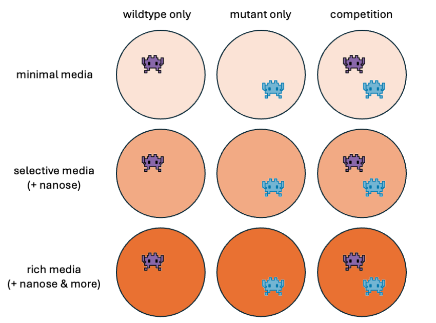
Your friend needs your help to analyze their Avida-Ed data. They designed a series of experiments around a mutant Avidian that gets an energy bonus when the sugar “nanose” is present and a wildtype Avidian that does not. They wanted to see how competition and resource availability affect the population dynamics of these Avidians.
Your friend grew either the wildtype only, mutant only, or both populations together (competition) in the following 3 environments:
Minimal (no additional sugars present)
Selective (only nanose present)
Rich (nanose and additional sugars present)
Help your friend get started with some of the exploratory data analysis. What relationships can you find between genotype, competition, and resource availability?
Data overview
Data for avida_wildtype.csv shown only:
| Column | Type | Description | Values |
|---|---|---|---|
update |
integer | Time elapsed | Ranges 0-300 |
condition |
character | Testing conditions (single population or competition) | Based off csv: wildtype-only, mutant-only, competition |
media_avg.fitness |
numeric | Average individual reproductive success in specified media | Ranges 0-1 |
media_avg.offspring.cost |
numeric | Average individual reproductive cost in specified media | |
media_avg.energy.acq.rate |
numeric | Average individual rate of energy acquisition from environment in specified media | |
media_pop.size |
integer | Population size in specified media | Ranges 0-900 |
All population measurements were determined for minimal, selective, and rich media.
Analysis ideas and hints
Which files have the pieces of data you need? Do you need to mix-and-match anything?
The data could be “tidier”…
Use these questions to develop your own or answer them as-is. There is no “single” or “correct” way to answer to these questions, and you can refine or broaden the scope of these questions as needed.
Bolded questions have an accompanying figure and code.
Easier
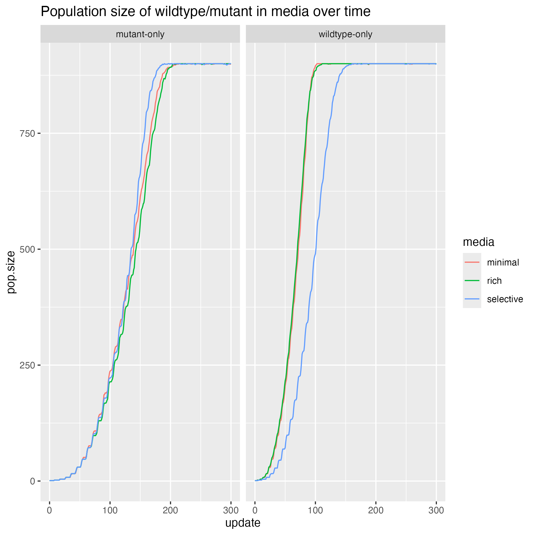
- How does population size change over time for the wildtype (or mutant) in different medias?
- What is the relationship between fitness and offspring cost in competition conditions in different medias?
Harder
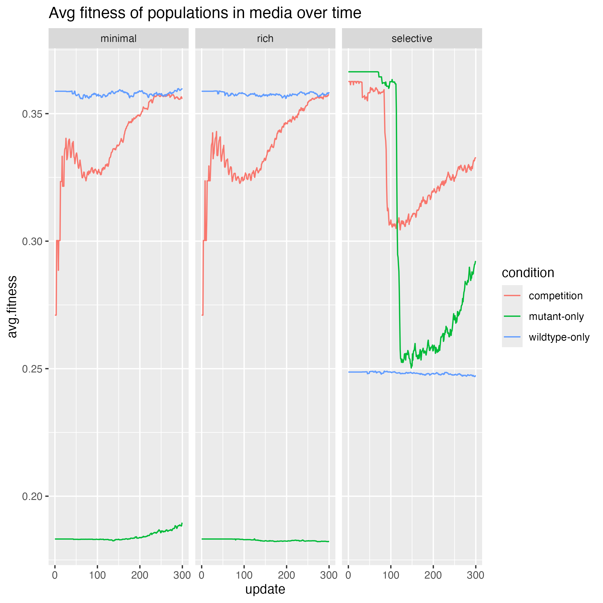
- How does the change in fitness over time compare between different treatment conditions and media types?
- Which media type allows for the most maximal performance of the wildtype? The mutant? Competition conditions?
Easier: How does population size change over time for the wildtype (or mutant) in different medias?
Harder: how does the change in fitness over time compare between different treatment conditions and media types?
Western Africa Ebola public health dataset
Skills to practice: working with dates, pivoting
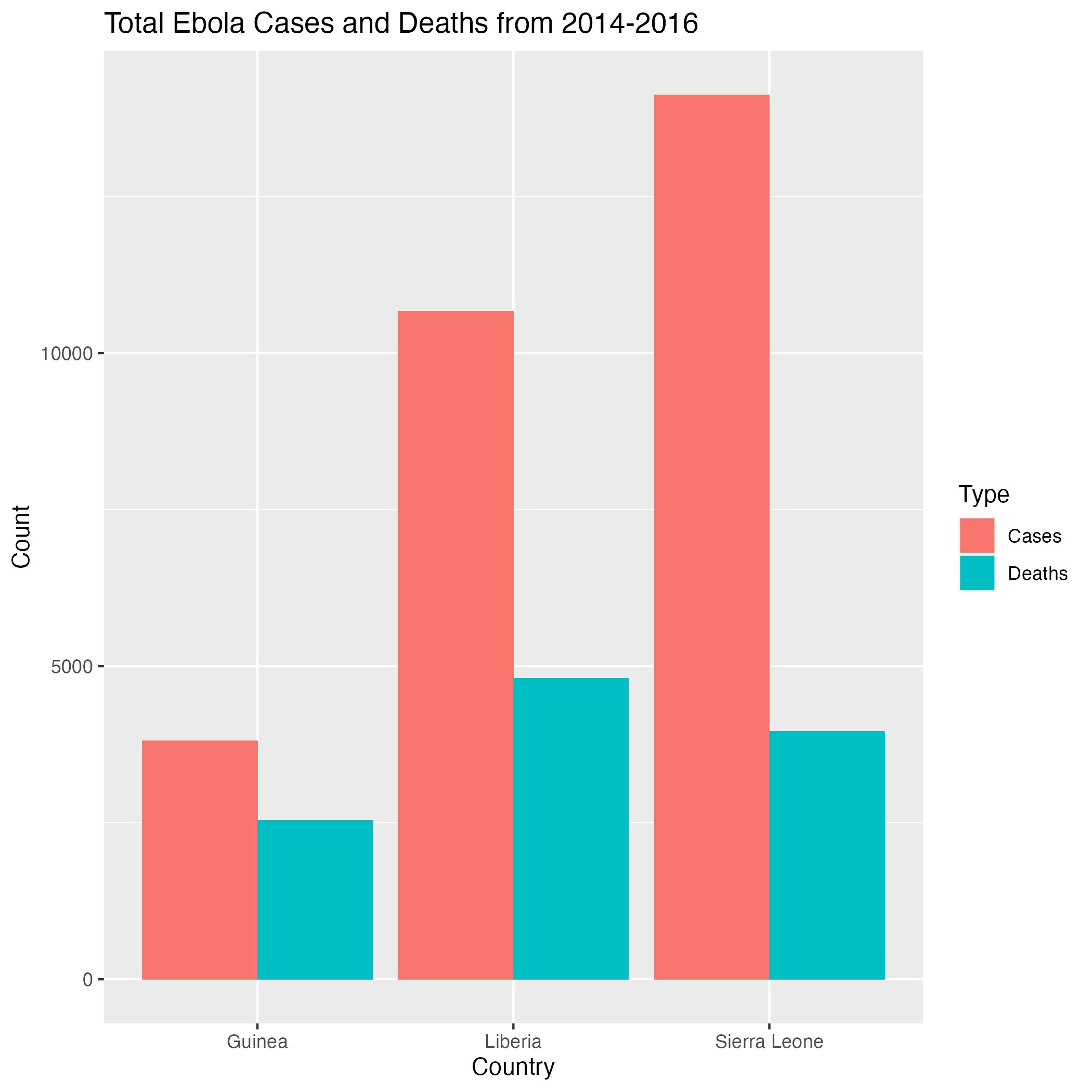
Background: The Western African Ebola virus (EV) epidemic of 2013-2016 is the most severe outbreak of the EV disease in history. It caused major disruptions and loss of life, mainly in the republics of Guinea, Liberia, and Sierra Leone.
How might you depict the dynamics of this outbreak?
Data overview
| Country | Date | Cumulative.no..of.confirmed..probable.and.suspected.cases | Cumulative.no..of.confirmed..probable.and.suspected.deaths |
|---|---|---|---|
| Guinea | 2014-08-29 | 648 | 430 |
| Nigeria | 2014-08-29 | 19 | 7 |
| Sierra Leone | 2014-08-29 | 1026 | 422 |
| Liberia | 2014-08-29 | 1378 | 694 |
| Sierra Leone | 2014-09-05 | 1261 | 491 |
| Nigeria | 2014-09-05 | 22 | 8 |
| Column | Type | Description | Values |
|---|---|---|---|
Country |
character | Country of report | |
Date |
character | Date of report | YYYY-MM-DD |
Cumulative.no..of.confirmed..probable.and.suspected.cases |
numeric | Cumulative number till this day | |
Cumulative.no..of.confirmed..probable.and.suspected.deaths |
numeric | Cumulative number till this day |
Analysis ideas and hints
This dataset contains data for other countries besides the three named above. For simplicity, you may want to focus on only those three regions.
The data could be “tidier”…
You can use
format()to extract specific parts of a date object: e.g. ifxis a date object with the format%Y-%m-%d, you can get the year withformat(x, "%Y").
Use these questions to develop your own or answer them as-is. There is no “single” or “correct” way to answer to these questions, and you can refine or broaden the scope of these questions as needed.
Bolded questions have an accompanying figure and code.
Easier
- How many cases and deaths in total were recorded by each country from 2014-2016?
- For a specific year, how did the number of cases and deaths change over time for each country?
Harder
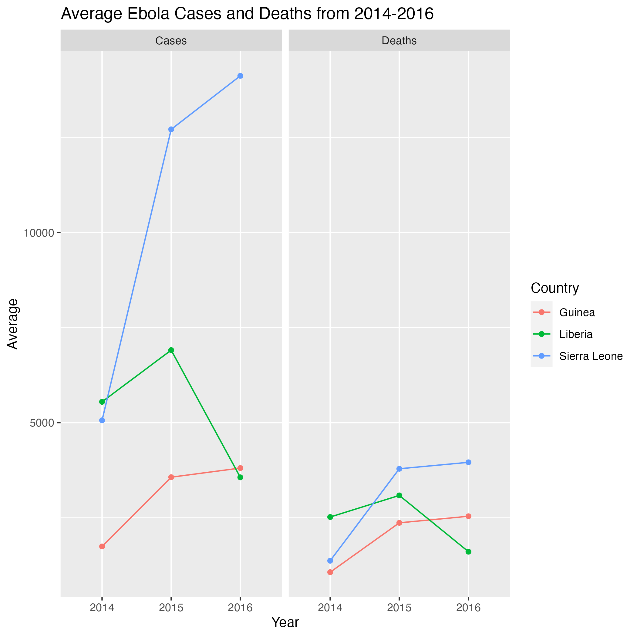
- By country, how did the average number of cases and death change each year?
- Are there any seasonal patterns in the average cases and deaths?
Easier: How many cases and deaths in total were recorded by each country from 2014-2016?
Harder: By country, how did the average number of cases and death change each year?
Heat exposure in Phoenix, Arizona ecological dataset
Data source | Related publication
Skills to practice: parsing strings, dealing with NA values
Background: Exposure to extreme heat is of growing concern with the rise of urbanization and ongoing climate change. Though most current knowledge about heat-health risks are known and implemented at the neighborhood level, less is known about individual experiences of heat, which can vary due to differences in access to cooling resources and activity patterns.
To further investigate, the Central Arizona-Pheonix Long-Term Ecological Research Program (CAP-LTER) recruited participants from 5 Pheonix-area neighborhoods to wear air temperature sensors that recorded their individually-experienced temperatures (IETs) as they went about their daily activities.
What relationships can you find between individual activity, temperature, and neighborhood?
Data overview
| Subject.ID | period | temperature |
|---|---|---|
| 1A | Sat, 8pm-12am | 25.14447 |
| 1P | Sat, 8pm-12am | 26.77962 |
| 1E | Sat, 8pm-12am | 27.21875 |
| 1B | Sat, 8pm-12am | 26.79175 |
| 2N | Sat, 8pm-12am | NA |
| 3A | Sat, 8pm-12am | NA |
| Column | Type | Description | Values |
|---|---|---|---|
Subject.ID |
character | Subject identifier where number (1-5) corresponds to neighborhood | 1=Coffelt, 2=Encanto-Palmcroft, 3=Garfield, 4=Thunderhill, 5=Power Ranch |
period |
character | 4 hour measurement period | weekday, period |
temperature |
numeric | 4 hour average of IET during specified period | Celcius |
Analysis ideas and hints
We recommend using functions in the
stringrpackage from the tidyverse to parse the strings, particularlystr_sub()andstr_split_fixed().e.g. If you had a vector
xcontaining a bunch of 2 character codes (XX), you could extract the first character withstr_sub(x, 1, 1).e.g. If you had a vector
xcontaining information in the formatfirst-second-third, you could extract that first chunk withstr_split_fixed(x, "-", n=3)[,1].
R has some “counting” functions such as
length()andn(): how could you get unique counts? Is there a single function that does that?
Use these questions to develop your own or answer them as-is. There is no “single” or “correct” way to answer to these questions, and you can refine or broaden the scope of these questions as needed.
Bolded questions have an accompanying figure and code.
Easier
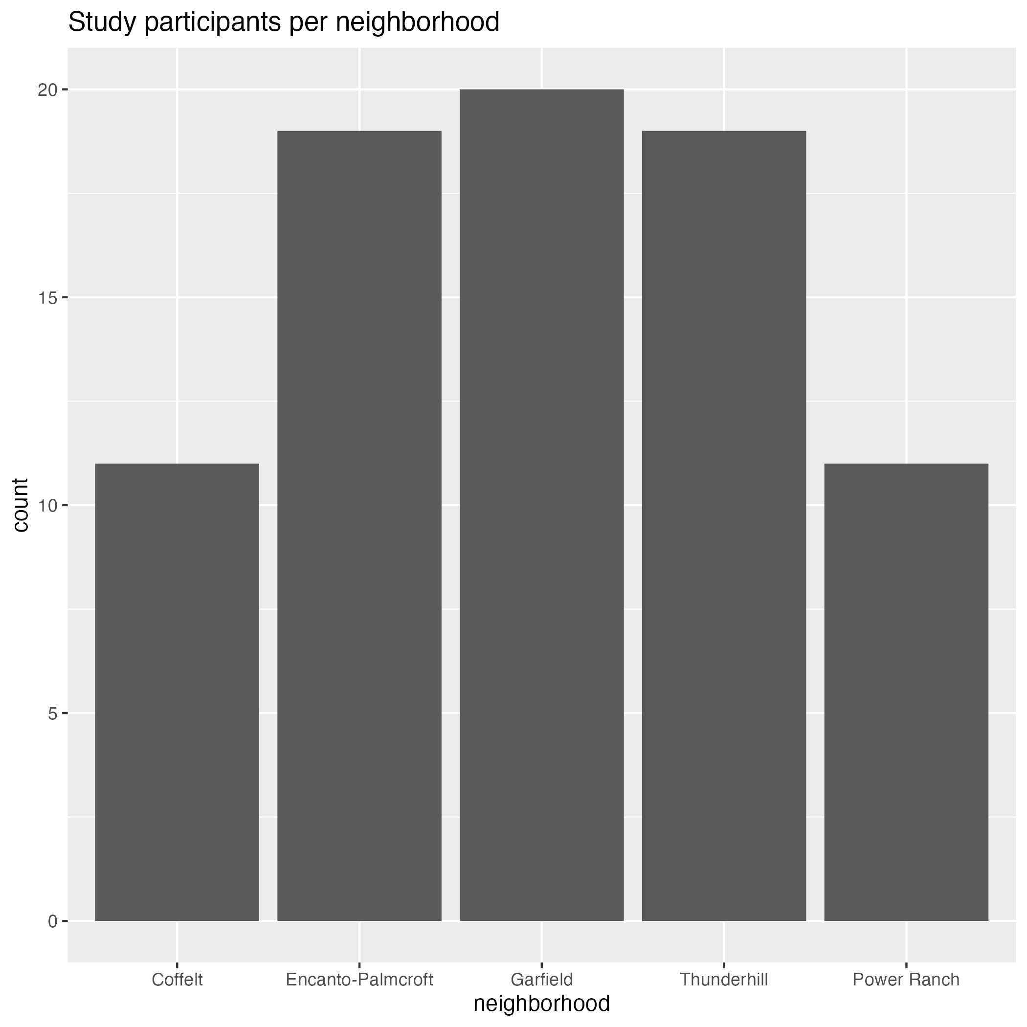
- How many participants were there for each neighborhood in the study?
- On average, which 4-hour measurement period is the warmest? The coolest?
Harder
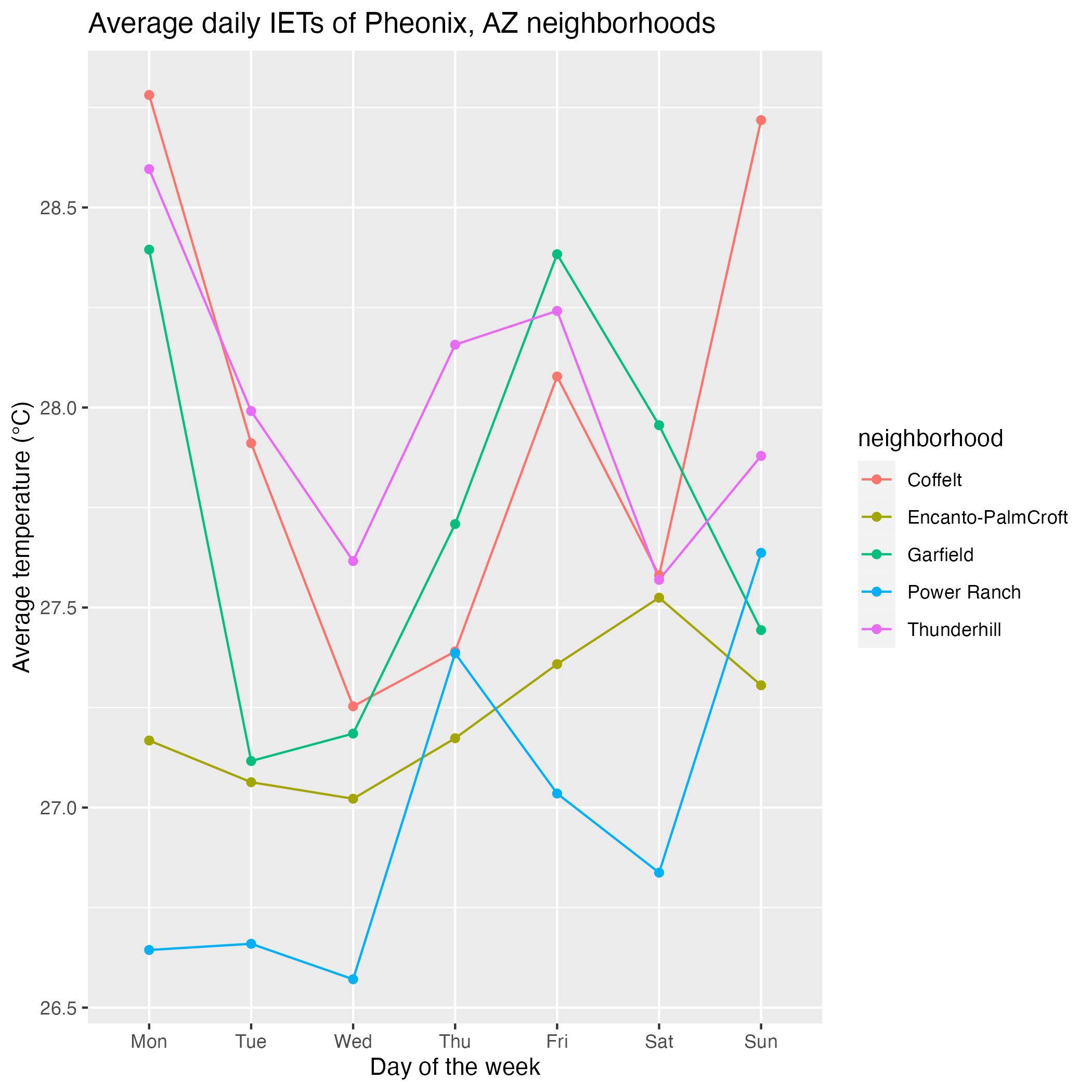
- What was the daily average temperature for each neighborhood during the study period?
- For a specific neighborhood on a specific day, what were all of the individual temperatures experienced for each 4-hour measurement period?
Easier: How many participants were there for each neighborhood in the study?
Harder: What was the daily average temperature for each neighborhood during the study period?
In particular, see Lenski et al. (2003) and Smith et al. (2016).↩︎